The Quantum Adoption Lifecycle: A 6-Stage Strategy for the NISQ Era


Executive Summary
Quantum computing is progressing from experimentation to structured adoption, where success depends on applying it to real business challenges. The Quantum Adoption Lifecycle provides the disciplined process that transforms research into cumulative capability. It guides organizations through six stages, from identifying where classical performance reaches its limits to developing quantum and hybrid solutions that deliver measurable value today and prepare for future fault tolerant systems. Each stage strengthens operational maturity: defining the problem in business terms, testing and validating approaches in controlled environments, optimizing through transpilation for current devices, and benchmarking results with integrity against the best classical and hybrid methods. The lifecycle enables organizations to move beyond isolated trials, focus investment where quantum truly adds advantage, and build adaptable solutions that evolve with advancing hardware.
Key Takeaways
- The Quantum Adoption Lifecycle transforms exploration into a disciplined capability-building process, creating reusable assets that scale as technology advances.
- Defines six actionable stages that convert experimentation into measurable business value through quantum and hybrid methods.
- Bridges the gap between architecture and execution: the Solution Stack defines the structure, while the Lifecycle provides the operational process that drives progress.
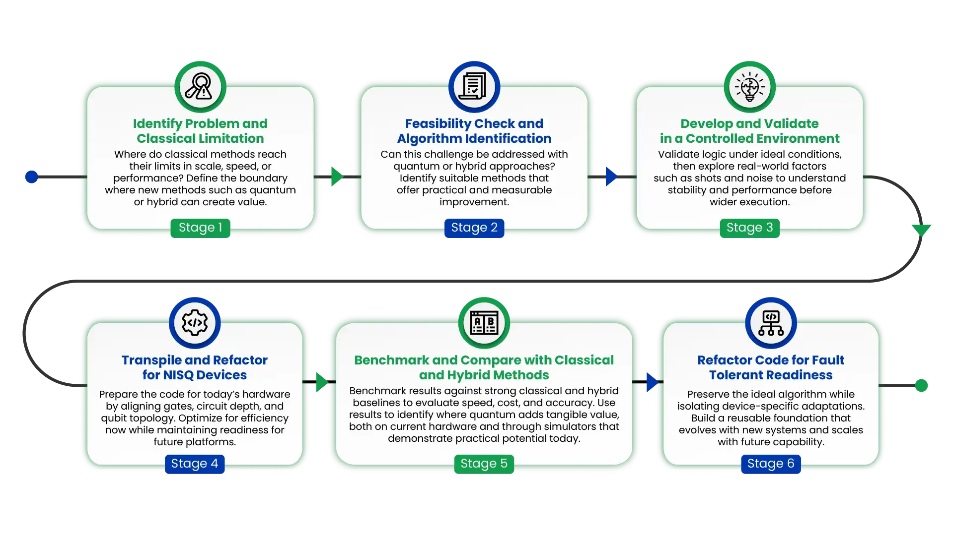
Figure: Strategy for Quantum Adoption in NISQ
Stage 1: Identify the Problem and Classical Limitation
Every quantum journey begins with asking where improvement is truly possible. The first stage identifies where classical computing reaches its limits in scale, speed, or precision. This means looking at the data – run times, accuracy trends, memory requirements, or model stability to pinpoint where added resources no longer produce useful gains.These provide clarity in understanding exactly where established methods stop delivering returns. In chemistry, this might be the point where molecular models become too large to simulate accurately. In optimization, it might be where the number of options grows faster than even advanced solvers can handle. In machine learning, it could be where adding data no longer improves accuracy. For technical and business leaders, this stage replaces intuition with quantifiable limits. A documented performance curve or cost threshold becomes the reference for every later experiment and gives a clear picture of where quantum approaches might create value.
Stage 2: Assess Feasibility and Identify the Right Approach
Once the boundaries of classical performance are clear, the next question is whether the challenge can be reframed in a way that quantum methods can handle, either alone or in a hybrid setting. This stage connects the business problem to the computational structure drawing from quantum areas such as simulation, optimization, or learning. It involves reviewing current research to understand what has already been proven, estimating the resources required, and judging whether experimentation with today’s hardware is practical. The result is a shortlist of viable pathways grounded in evidence.
Stage 3: Develop and Validate through Simulators
With a potential approach identified, this stage focuses on validation in a controlled environment before moving to real hardware. Development begins in a simulator to confirm that the logic works under ideal conditions, then progressively incorporates practical factors such as sampling and noise. Hardware profiles are examined to understand qubit connectivity, gate error rates, and coherence times and incorporated into the simulator using available noise function generators. This structured validation confirms stability and performance under realistic conditions and prepares the design for hardware execution.
Stage 4: Adapt for Near-Term Devices
At this point, the design is translated into an executable form suited for today’s quantum hardware. The circuit is transpiled and compiled for the target backend so that it aligns with the device topology, native gate sets, and connectivity constraints. The objective is to stay within coherence limits while balancing fidelity and practicality, reducing circuit depth, limiting costly multi-qubit operations, and arranging qubits to minimize routing overhead. Throughout this process, it is essential to maintain a clear separation between the core logic and device-specific adjustments so that the design remains portable and can be retargeted as hardware improves.
Stage 5: Benchmark and Compare with Classical and Hybrid Methods
Performance is evaluated against strong classical baselines to understand the true contribution of quantum methods. Comparisons cover accuracy, runtime, and computational cost, using consistent datasets and metrics to ensure credibility. In addition to classical baselines, benchmarking also opens the possibility to explore solutions that can run effectively on classical hardware today while still applying quantum principles. This allows meaningful progress and value creation without waiting for fault tolerant and large scale quantum systems.The goal is not only to find better solutions, but to gain deeper insight. Benchmarking provides context, showing where quantum approaches align with, extend, or complement classical performance. It highlights both strengths and current gaps, turning results into insight and guiding further design toward practical and scalable quantum advantage.
Stage 6: Prepare for Fault Tolerant and Future Readiness
Each experiment should leave behind a durable foundation. In this stage, the solution is refined so that it remains relevant as technology advances. Core logic is separated from device-specific tuning, code and configurations are archived clearly, and results are documented for reproducibility. This stage turns each project into a reusable building block for later work. As algorithms mature and hardware improves, these validated assets become the foundation of larger programs that advance steadily toward fully error-corrected quantum computing.
Case Studies: Applying the Lifecycle
We cover three examples to show how the six-stage Quantum Adoption Lifecycle can be applied across distinct problem classes. Each illustrates how a structured process turns exploration into repeatable capability. The details of algorithms, baselines, and configurations provided below are examples for illustration, while the main motive is to show how each follows the same disciplined rhythm: define limits, study the feasibility, validate performance, benchmark with integrity, and build continuity for future systems.
Example 1 – Simulation: Molecular Energy Estimation
Stage 1: Identify the Problem and Classical Limitation
In quantum chemistry, calculating molecular energy quickly becomes costly as molecular size grows. Classical coupled-cluster methods such as CCSD(T) exhibit O(N⁷) scaling, which limits exploration of larger molecules. Measurements of runtime and accuracy show the classical ceiling clearly.
Stage 2: Assess Feasibility and Identify the Right Approach
The problem is reframed as a ground-state energy estimation within a molecular Hamiltonian. The Variational Quantum Eigensolver is chosen because it combines quantum precision with classical optimization. Resource estimates show that small molecules can already be explored with current devices.
Stage 3: Develop and Validate through Simulators
Hamiltonians are encoded through Jordan-Wigner and Bravyi-Kitaev mappings. Various ansatz structures are simulated to test expressivity versus circuit depth. Optimizers such as COBYLA and SPSA are benchmarked for convergence stability. Noise-model simulations reveal how hardware imperfections influence accuracy.
Stage 4: Adapt for Near-Term Devices
Circuits are compiled for the selected backend. Depth and layout are tuned to remain within coherence limits. Gate scheduling, qubit mapping, and simple error-mitigation steps are applied.
Stage 5: Benchmark and Compare with Classical and Hybrid Methods
Quantum energy estimates are compared with established classical references such as FCI and CCSD(T). Simulators provide a way to evaluate performance today, using classical resources to test quantum algorithms and understand where they already add value. Observed results on simulated quantum methods achieving chemical accuracy for small molecules are used to indicate where scaling begins to offer efficiency gains. Benchmarking highlights both progress and current limits, guiding refinement toward practical quantum-ready chemistry.
Stage 6: Refactor for Fault Tolerant Readiness
All data, mappings, and configurations are archived in portable form with complete metadata. The framework is reusable for larger molecules and compatible with future devices offering longer coherence and lower error.
Example 2 – Optimization: Supply Chain Scheduling
Stage 1: Identify the Problem and Classical Limitation
Complex supply chains generate an enormous number of possible schedules. Classical solvers struggle to adjust dynamically when routes or constraints change. Benchmarking solver performance against network size identifies the classical boundary where responsiveness declines.
Stage 2: Assess Feasibility and Identify the Right Approach
The scheduling challenge is modeled as a Quadratic Unconstrained Binary Optimization problem. The Quantum Approximate Optimization Algorithm is selected for its ability to represent cost functions efficiently. Feasibility tests confirm that modest instances can be handled on present systems.
Stage 3: Develop and Validate through Simulators
Simulation examines how circuit depth, parameter settings, and cost-function scaling affect solution quality. Parameter sweeps and noise-model studies identify configurations that balance accuracy with runtime.
Stage 4: Adapt for Near-Term Devices
Circuits are compiled for hardware with limited qubit connectivity. Gate reduction and mapping strategies are used to fit coherence times. Classical processing handles pre- and post-optimization steps, enabling practical hybrid execution.
Stage 5: Benchmark and Compare with Classical and Hybrid Methods
Results are compared with solvers like CP-SAT, simulated annealing, and genetic algorithms. Simulators help test quantum formulations on classical hardware to reveal where they improve exploration or convergence. Insights show where quantum methods begin to offer measurable benefits.
Stage 6: Refactor for Fault Tolerant Readiness
The Hamiltonian formulation, data encodings, loss constraints, and orchestration scripts are modularized and stored for reuse. These modules scale with larger networks as hardware capability and gate fidelity increase.
Example 3 – Quantum for AI: Financial Anomaly Detection
Stage 1: Identify the Problem and Classical Limitation
Detecting fraud in financial data requires finding subtle, nonlinear patterns among millions of transactions. Classical models reach limits of recall and precision when data imbalance becomes extreme. Precision–recall curves provide clear evidence of that plateau.
Stage 2: Assess Feasibility and Identify the Right Approach
A hybrid quantum–classical design is created. Quantum feature maps expand the data representation before classification by support-vector machines or neural networks. Early studies show that quantum kernels can capture patterns that classical kernels overlook.
Stage 3: Develop and Validate through Simulation
Encoding methods including angle, amplitude, and phase are tested to measure separability of anomalies. Controlled runs with realistic noise confirm stability and predictive accuracy.
Stage 4: Adapt for Near-Term Devices
Compact feature-map circuits are compiled for available hardware. Parameter tuning maintains expressivity while keeping depth minimal. Integration with classical analytics pipelines ensures inference latency remains practical.
Stage 5: Benchmark and Compare with Classical and Hybrid Methods
Quantum-enhanced models are benchmarked against classical baselines using proper dataset splits and reproducible seeds. Improved metric scores such as recall and precision translate directly into fewer missed fraud cases and reduced cost of false alerts.
Stage 6: Refactor for Fault Tolerant Readiness
The full workflow, including data-encoding templates and classifier parameters, is stored as a reusable framework. It can adapt to new datasets and larger circuits as quantum capacity improves.
Across industries and problem domains, the Quantum Adoption Lifecycle turns quantum exploration into structured progress. It builds a foundation of reusable capability, measurable improvement, and strategic readiness for the next generation of computing. Successive iterations convert learning into capability and moves closer to practical quantum utility.
Conclusion
The Quantum Adoption Lifecycle provides a structured, repeatable approach to build, refine, and scale quantum solutions with clarity and discipline. It turns isolated experiments into a continuous cycle of measurable progress, creating a foundation for long-term capability and value. Each iteration strengthens organizational knowledge, enhances classical and hybrid comparisons, and moves the enterprise closer to practical quantum advantage. In upcoming posts, we will show this lifecycle in action, demonstrating how it can be applied step by step to real business problems.